Creating and Modifying Forecasts

Configuration Process Understanding MRP Bucket Types and demand impact Using historical and seasonal forecasts Utilizing the "Same As" and "% Increase" functionalities Using Time-Phased vs Instant MRP reports Creating the Forecast Creating Forecasts Using Moving Average and Weighted Moving Average Entering Moving Average Forecasts Entering Weighted Moving Average Forecasts Entering Moving and Weighted Moving Average Forecasts for Seasonal Items Creating Forecasts Using Linear Regression Linear Regression Forecast Example Creating Forecasts Using Simple, Double, or Triple Exponential Smoothing Simple Exponential Smoothing Example Double Exponential Smoothing Example Triple Exponential Smoothing Example FAQ & Diagnostic Tips

Forecasts allows users to easily create and modify forecasts to assist with production and sales management. In DEACOM, sales forecasts are used to drive the MRP process. Active forecast sheets setup demand in the "(-M) forecast" demand bucket in time-phased MRP. Forecasts can be leveraged to:

• Create sales forecasts based on historical sales of items in DEACOM.
• Update existing sales forecasts by utilizing the percentage change tool and the pre-filter capabilities.
• Compare forecast sheets to actual sales.

Configuration

The configuration steps necessary are covered in the Process section below.

Process

Forecasts can be setup based on historical sales or manually by a user. Parts included on these forecasts can be grouped together by product category, sales rep, Facility, etc., depending on company operations. Prior to creating a Forecast, it is important to understand the various options and impacts they have in DEACOM. These options are described below, followed by information on how to manage Forecasts.

Understanding MRP Bucket Types and demand impact

The Edit Forecast form contains an "MRP Bucket Type" field which determines how the Forecast will be applied to MRP reports. These options, explained by the "MRP Bucket Type" field description on the Forecasts page, are Days, Weeks, and Months. Forecasts may be created for short-term demand or long-term, depending on the product/customers. While this bucket size may vary, the maximum number of buckets allowed in DEACOM is 60.

As far as demand impact, Forecasts are generally created prior to real Sales Orders. it is important to note that Purchase Orders may also be created and linked to a specific Sales Order. In the event that both Forecasts and Purchase Orders exist for a given sale, MRP will take the net of Forecasts and ordered Parts. For example, if a Forecast exists for 100 units and a Purchase Order exists for 40 units, MRP will calculate a net of 60 units, indicating that that amount must be purchased or produced to meet current demand.

Using historical and seasonal forecasts

Companies will often use historical sales information for the basis of future sales forecasts. The “Create Forecast” button on the following sales order reports is used to create historical forecasts.

• Sales order detail
• Sales User detail 1-5
• Sales User summary 1-5

When using this option, the system displays the items and item quantities shipped on sales orders to allow the user to create a new forecast sheet.

• Note: Inter-Company Transfers are not included in historical sales since they are not invoiced. The steps necessary to create a historical forecast are indicated in the Creating the Forecast section below.

Once historical forecasts are created, the "Forecast vs Actual" report type, via Sales > Forecasts, can be used to compare a sales forecast to historical sales, and therefore analyze the actual sales performance based on a selected forecast sheet. 

Many industries experience seasonal demand based on a variety of factors. Generally speaking, seasonal demand has a pattern that repeats. For example, demand for clothing has a seasonal pattern that repeats every 12 months. There could also be seasonality on a smaller time scale, such as per week. Once a forecast has been created, users may use the "Same As" button, described below, to create a copy that can then be modified and saved to represent seasonal changes on individual items or groups of items. The "% Increase" button, also described below, allows users to quickly establish quantity adjustments based on seasonal changes.

Utilizing the "Same As" and "% Increase" functionalities

The "Same As" button on the Edit Forecast form allows an existing forecast sheet to be copied into a new Forecast sheet. This functionality can be very useful because DEACOM does not store historical copies of forecast sheets (to minimize database storage space). Prior to making an update to an original Forecast sheet, a copy of that forecast sheet can be made so that the original can be compared to actual sales at any point during the year. To create a new forecast sheet follow the steps below:

1. In the Forecasts pre-filter, set the "Forecast Source" field to Manual and then click the "View" button.
2. In the Edit Forecast form, click the "Same As" button and select the original forecast sheet which will be copied.
3. On the subsequent Edit Forecast form, enter an appropriate name for the forecast sheet then click the "Save" button.

The "% Increase" button, also on the Edit Forecast form, can be used to apply an increase to one or all periods of the selected forecast. The percent increase is applied to only the portion of the sales forecast shown in the grid. Thus, if results are filtered through the pre-filter, the percent increase is only applied to the filtered results and the items left off the filtered forecast sheet are not updated. A couple items of note regarding percent increases:

• This option also allows a user to specify a negative factor, which will decrease the results by the value entered.
• All increases/decreases applied are stacked. So, if an increase is applied to one month then another increase is applied to all buckets, that one month chosen will get increased twice.

Using Time-Phased vs Instant MRP reports

Active forecast sheets and active Forecast Sales Orders Types setup demand in the "(-M) forecast" demand bucket in time-phased MRP. The differences in how MRP displays data in Time-Phased vs Instant MRP is discussed on the "MRP" page.

Once MRP reports are displayed users can drill into the "(-M) forecast" line or column to see the name of the Forecast or order number of the Forecast Sales Order. From here, the "View Detail" button can be used to drill into the Forecast or Forecast Sales Orders themselves.  When drilling into the Forecast line of column, the system will filter the drill-down screen to only show the forecast buckets that are applicable to the amount and date range shown in MRP. 

Creating the Forecast

Typically, organizations will create a forecast sheet using historical sales. To do so, perform the following:

1. Navigate to Sales > Order Reporting.
2. On the pre-filter select a report type of Order Detail (or Sales User Detail 1-5 or Sales User Summary 1-5) and an appropriate start date.
3. Fill in the rest of the pre-filter with the appropriate criteria.
4. Click the “View” button to generate the report.
5. On the report click the “Create Forecast” button to display the Create Forecast form.
6. The "Forecast Start" date will be defaulted based on the start date selected on the Sales > Order Reporting pre-filter. It can be changed here if necessary.
7. Select appropriate values for the “Bucket Type” and “Number of Buckets” fields. These fields determine the bucket period and length of the forecast sheet. See the Forecasts page for field descriptions.
   • The user can also optionally select to group the forecast lines according to Bill-To, Ship-To, or Facility with the respective checkboxes.
8. Once complete, click the “Continue” button to display the Edit Forecast form.
9. Add new or modify existing lines based on the forecast purpose. A new part can be added to an existing forecast sheet by using the "Add" button on the Edit Forecast form and an existing line can be modified by using the "Modify" button. Both display the same Edit Forecast Line form, which allows a user to manually create/update the forecast line.
   • On the Edit Forecast Line form, the scaling tools (selected using the "Change Type" pick list) may be used to update the selected Forecast line.
   • In addition, items can be assigned to a Customer by selecting the appropriate record(s) in the corresponding fields. When calculating forecast sums for a part in MRP, the system will also sum the forecast lines assigned to a specific Bill-to or Ship-to.
   • Users can enter multiple entries for the same part on the same forecast, as long as the Bill-to, Ship-to, and/or Facilities on the entries are different.
10. Once all selections have been made on the Edit Forecast Line form, click "Save".
11. Click "Next" to add more forecast lines or "Exit" to return to the Edit Forecast form.
12. Review the overall forecast and ensure it is accurate, then click "Save" to complete the process.

Note: In DEACOM, forecast quantities are represented in the item's stock unit of measure.

Creating Forecasts Using Moving Average and Weighted Moving Average

Beginning in version 16.06.011 users have the option to create Forecasts using moving average and weighted moving average logic. Details regarding the logic are available in the Create Forecasts section. The steps necessary to enter moving average forecasts are listed below.

Entering Moving Average Forecasts

1. Navigate Sales > Order Reporting and select a Report Type of order detail or a Sales User Detail 1-5 report.
2. Click the "Create Forecast" button to display the Create Forecast form.
3. Select "Moving Average" Forecast Method.
4. Fill out all the necessary fields on this form.
5. Press the "Continue" button to display the "Edit Forecast" form. The grid is populated with the appropriate values. Additional details on how the form is populated can be found on the Create Forecasts page.
6. Modify or verify the information as necessary and save the Forecast when complete. Note that users may use the "Apply Smoothing" button if desired. In this case, the "Create Forecast" form will appear with the historical data start date already filled in. At this point, users can select “Weighted moving average” in forecast method and fill in the rest of the required fields. Once the "Continue" button is pressed, the forecast will be updated with the newly calculated weighted moving average values.

Entering Weighted Moving Average Forecasts

1. Navigate Sales > Order Reporting and select a Report Type of order detail or a Sales User Detail 1-5 report.
2. Click the "Create Forecast" button to display the Create Forecast form.
3. Select "Weighted Moving Average" Forecast Method.
4. Fill out all the fields on this form. Note that the number of periods indicated must not be prior to the Historical Start Date otherwise the user will be prompted with "The number of periods considered can’t use buckets prior to the historical start date. Update the number of periods, or dates to continue."
5. Press the "Continue" button to display the "Enter Bucket Weights" form.
6. The system will display with the option to enter values for the bucket weights based on the forecast start and the periods considered. Enter the appropriate weights. Note that weights must add up to 100%.
7. Press the "Continue" button to display the "Edit Forecast" form. The grid is populated with values calculated using a weighted moving average for each bucket based on the weights entered.
8. Modify or verify the information as necessary and save the Forecast when complete. Note that users may use the "Apply Smoothing" button if desired. In this case, the "Create Forecast" form will appear with the historical data start date already filled in. At this point, users can verify or modify information in the appropriate fields. Once the "Continue" button is pressed, the forecast will be updated with the newly calculated values.

Entering Moving and Weighted Moving Average Forecasts for Seasonal Items

1. Navigate Sales > Order Reporting and select a Report Type of order detail or a Sales User Detail 1-5 report.
2. Click the "Create Forecast" button to display the Create Forecast form.
3. Select ""Moving Average" or Weighted Moving Average" Forecast Method.
4. Fill out all the fields as required. To generate a new forecast form past data you would fill out the Create Forecast form similar to this example below:
   1. Forecast Method: Moving Average
   2. Forecast Start Date: 01/01/2024
   3. Historical Data Start: 01/01/2023
   4. Bucket Type: Months
   5. Number of Buckets: 3
   6. Periods Considered: 3
5. Press the "Continue" button to display the "Edit Forecast" form. The grid is populated with the appropriate values.
6. Modify or verify the information as necessary and save the Forecast when complete. Note that users may use the "Apply Smoothing" button if desired. In this case, the "Create Forecast" form will appear with the historical data start date already filled in. At this point, users can verify or modify information in the appropriate fields. Once the "Continue" button is pressed, the forecast will be updated with the newly calculated values.

Creating Forecasts Using Linear Regression

Beginning in version 16.06.013 users have the option to create Forecasts using linear regression. The necessary steps are detailed below.

1. Navigate Sales > Order Reporting and select a Report Type of order detail or a Sales User Detail 1-5 report.
2. Click the "Create Forecast" button to display the Create Forecast form.
3. Select "Linear Regression" Forecast Method.
4. Fill out all the necessary fields on this form. Note that the number of periods indicated must not be prior to the Historical Start Date otherwise the user will be prompted with "The number of periods considered can’t use buckets prior to the historical start date. Update the number of periods, or dates to continue." Also, Linear Regression requires at least 3 buckets of historical data prior to the forecast start.
5. Press the "Continue" button to display the "Edit Forecast" form. The grid is populated with the appropriate values. Additional details on how the form is populated can be found on the Create Forecasts page.
6. Modify or verify the information as necessary and save the Forecast when complete. Note that users may use the "Apply Smoothing" button if desired. In this case, the "Create Forecast" form will appear with the historical data start date already filled in. At this point, users can verify or modify information in the appropriate fields. Once the "Continue" button is pressed, the forecast will be updated with the newly calculated values.

Linear Regression Forecast Example

	Title	time(x)	Sales(y) f2_origquant	xy	x^2	Forecast-f2_quant
Historical Start
	Bucket	1	600	600	1	0
	Bucket	2	1550	3100	4	0
	Bucket	3	1500	4500	9	0
	Bucket	4	1500	6000	16	0
	Bucket	5	2400	12000	25	0
	Bucket	6	3100	18600	36	0
	Bucket	7	2600	18200	49	0
	Bucket	8	2950	23200	64	0
	Bucket	9	3800	34200	81	0
	Bucket	10	4500	45000	100	0
	Bucket	11	4000	44000	121	0
	Bucket	12	4900	58800	144	0
	Sum	78	33350	268200	650
	Avg	6.5	2779.17
Forecast Start
	Bucket	13	0			5116.57
	Bucket	14	0			5476.17
	Bucket	15	0			5835.77
	Bucket	16	0			6195.37

Based on the above data, you can see that the forecast starts on bucket# 13, with historical buckets being 1-12.

• Time (x) represents the bucket numbers, and y is the forecast quantities in f2_origquant (historical sales)

• The equation used to generate the new forecast quantity will be y = a + b(x)
  • b = (268200 - 12 × 6.5 × 2779.17)/ (650 – 12 × [6.5]^2 )              b = 359.6
  • 268200 = bucket# X quantity sold
  • 12 = total buckets
  • 6.5 = total buckets summed (78) / how many buckets
  • 2779.17 = average quantity sold
  • 650 = bucket number squared
  • a = 2779.17 - 359.6 × 6.5             a = 441.77
  • bucket 13 = 441.77 + 359.6 × 13 = 5116.57
  • bucket 14 = 441.77 + 359.6 × 14 = 5476.17
  • bucket 15 = 441.77 + 359.6 × 15 = 5835.77
  • bucket 16 = 441.77 + 359.6 × 16 = 6195.37

Creating Forecasts Using Simple, Double, or Triple Exponential Smoothing

1. Navigate to Sales > Order Reporting and select a Report Type of order detail or a Sales User Detail 1-5 report. (Note: Simple, Double, and Triple Exponential Smoothing forecasts may also be created via the "Apply Smoothing" button when modifying an existing Forecast)
2. Click the "Create Forecast" button to display the Create Forecast form.
3. Select either "Simple Exponential Smoothing", "Double Exponential Smoothing", or "Triple Exponential Smoothing" in the Forecast Method.
4. Fill out all the necessary fields on this form. Note that at least 2 full periods of historical data are required to generate a forecast using exponential smoothing.
5. Press the "Continue" button to display the "Forecast Weight" form in order to enter smoothing constants.
6. Fill in the appropriate value for the Alpha, Beta, and Gamma fields and choose either a Multiplicative (default) and Additive
7. Click "Continue" to apply the changes.
8. Modify or verify the information as necessary and save the Forecast when complete.

Simple Exponential Smoothing Example

Sales order detail data shipped from 10/01/2020 - 02/01/20201. Example using a single part to simplify. Forecast Created on 02/01/2020, and some orders had shipped on the first. Therefore, we have an f2_origquant in February, but it will not be considered.

• Historical Start - 10/01/2020
• Forecast Start - 02/01/2021
• Forecast Bucket - Months
• Number of Buckets – 3 (This means we will have 3 buckets from 02/01/2021 forward)
• Smoothing Constant (alpha) - 0.5

We must first calculate forecasts for all buckets from the historical start date, to then generate new forecasts into the f2_quant field for buckets after the forecast start date.

Formula:

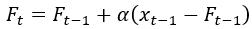
F = Forecast

α = Smoothing Constant

x = Actual Sales

t = bucket (time)

The forecast for the 1st period is assumed to be the actual, since we don't have a forecast quantity calculated. Simple exponential smoothing will result in the same forecast value for all buckets after the forecast start date. 

Lastly calculate the mean absolute percent error (MAPE) for each forecast line, and pop

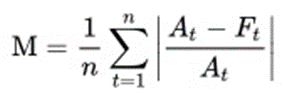
M = mean absolute percent error

n = number of times the summation iteration happens

A(t) = actual value

F(t) = forecast value

Bucket	Month	f2_origquant	f2_quant	Calculation	Error
1	Oct	20		20 – Set equal to actual
2	Nov	27		20 + 0.5(20-20) = 20	35
3	Dec	33		20 + 0.5(27 -20) = 23.5	28.78
4	Jan	45		23.5 + 0.5(33 – 23.5) = 28.25	37.22
5	Feb	6	36.63	28.25 + 0.5(45-28.25) = 36.625
6	March	0	36.63	N/A
7	April	0	36.63	N/A
					MAPE = 33.67

Double Exponential Smoothing Example

• Forecast Created on 02/01/2020
• Historical Start – 04/01/2020
• Forecast Start - 02/01/2021
• Forecast Bucket - Months
• Number of Buckets – 5 (This means we will have 3=5 buckets from 02/01/2021 with an f2_quant)
• Smoothing Constant (alpha) - 0.7
• Trend Smoothing Constant(beta) – 0.6

Formula:

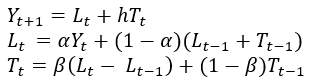
Y = Forecast

L = Level

T = Trend

h = forecast horizon (used in future buckets)

t = bucket number

α = Level Smoothing Constant

β = Trend Smoothing Constant

First calculate forecasts for all buckets from the historical start date, to then generate new forecasts into the f2_quant field for future buckets. We will need at least 2 historical buckets to calculate a forecast.

We will need to unitize values for level and trend. To simplify this

• Set level of bucket 2 = sales in bucket 2
• Set trend of bucket 2 = Bucket 2 Sales – Bucket 1 Sales

Establishing the trend this way requires 2 previous buckets of historical data, which is why we require them. Now that we have established a level and trend in bucket 2, we can create our first forecast for bucket 3. Use the standard forecast formula.

The normal trend and level equations can now be used to calculate trend and level for all buckets containing historical data.

When projecting the forecast beyond 1^st forecast bucket, we will continue to use the last values for trend and level. The horizon(h) will increment up by 1 for each bucket. In this example 1-5 is used for the 5 forecast buckets. June 2021 formula = 22.76 + (5) * 2.62 = 38.56

Lastly calculate the MAPE for each forecast line and populate into f2_stderror.

Bucket	Month	F2_origquant	F2_quant	Level	Trend	Forecast	Error
1	April 2020	6.4	0	N/A	N/A	N/A
2	May 2020	5.6	0	5.6 Set = Actual	-0.8 =5.6-6.4	N/A
3	June 2020	7.8	0	6.9	0.46	4.8 =5.6 + -0.8	38.46
4	July 2020	8.8	0	8.37	1.06	7.36 = 6.9 + 0.46	18.46
5	August 2020	11	0	10.53	1.72	9.43	14.27
6	September 2020	11.6	0	11.8	1.45	12.25	5.60
7	October 2020	16.7	0	15.66	2.9	13.24	20.72
8	November 2020	15.3	0	16.28	1.53	18.56	21.31
9	December 2020	21.6	0	20.46	3.12	17.81	17.55
10	January 2021	22.4	0	22.76	2.62	23.58	5.26
11	February 2021	4	25.38		h = 1	25.38
12	March 2021	0	28.00		h = 2	28.00 = 22.76+(2*2.62)
13	April 2021	0	30.63		h = 3	30.63
14	May 2021	0	33.25		h = 4	33.25
15	June 2021	0	35.88		h = 5	35.88
							17.70 = Avg all errors for MAPE =

Triple Exponential Smoothing Example

• Forecast Created on 02/01/2020
• Historical Start – 01/01/2018
• Forecast Start – 01/01/2018
• Forecast Bucket – Months
• Number of Buckets – 12 (can be less than a period)
• Buckets In A Period - 12
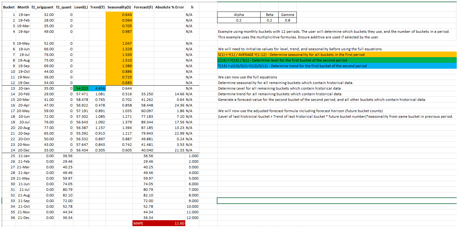
• Smoothing Constant (alpha) - 0.2
• Trend Smoothing Constant(beta) – 0.2
• Seasonality Smoothing Const(gamma) – 0.2
• Formula Type – Multiplicative 

Triple Exponential can be done using a multiplicative or additive formula. Use the formula selected by the user when they generate the forecast or apply smoothing.  

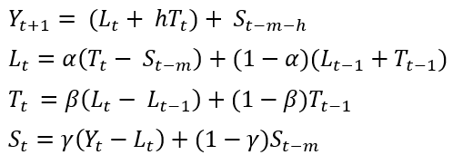
Multiplicative Formula:

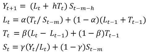
m = Seasonal period. In a monthly forecast m = 12, weekly m = 52, daily m = 365.

Additive Formula:

FAQ & Diagnostic Tips

If a Forecast is created via the Order Entry function, can it be modified via Forecasts and vice versa?

No, because the Forecast Sales Order does not have a name and the Forecast does not have a Sales Order number. A Forecast must have a name in order to view/modify it in Forecasts or an order number to view/modify it in Sales > Order Reporting

Can sales forecasts be displayed in Financial Statements?

Yes, beginning in version 16.00.087, the "Forecast" field, available on the Generate Financial Statement form can be used to display forecast amounts when  the start and end dates of the statement are within the range of the Forecast and the revenue accounts specified on item master records contained in the Forecast match the revenue accounts specified on the statement line.